Student Manual
PAGE 6
There are over 200 galaxies in our sample. For the purposes of this exercise, you can assume that this is all the galaxies
that we can see through the telescope. In fact there are many more than this in the real sky, but we have omitted many to
make the measurement task less tedious. This isn’t that unrealistic, because even under the best conditions, astronomers’
catalogs of galaxies never can include all the galaxies in a given volume of space. Faint galaxies, or ones which are
spread out loosely in space may be hard to see and may not be counted. Still, our sample contains enough galaxies to
show the large-scale features of the visible universe in this direction. It is your assignment to discover those features for
yourselves.
Even 200 galaxies is a lot to investigate in a single class period. Your instructor may have you do the assignment in one
of several ways. You may work in small groups, each group observing a 20 galaxies or so during the first part of the class.
The groups can then pool their data together into one combined data set to produce a single map for your analysis. This
group effort is the way most astronomers work—they collaborate with other astronomers to turn large unmanageable
projects into smaller, manageable tasks. You may compile and analyze the data during several class periods. Or, you
may be doing this lab as a term project or out-of-class exercise.
This write-up assumes you will be following strategy number 1, that is you’ll be one of several
groups working collaboratively to pool data. We’ll assume
you’re going to obtain spectra of 20 galaxies which you
will later combine with other groups to get redshifts of
all 218 galaxies in our sample. Though we have
provided work-sheets for only 20 galaxies in
this write-up, you can still use this write-up
as a guide even if you are measuring all 218
galaxies yourself.
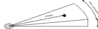
The region you’re going to be examining is shape like a thick piece of pie, where the thickness of the pie slice is the
declination, and the length of the arc of crust represents the right ascension. The radius of the pie, the length of the slice,
is the furthest distance included in the survey.
Technical Details
How does the equipment work? The telescope can be pointed to the desired direction either by pushing buttons (labeled
N,S,E,W) or by typing in coordinates and telling the telescope to move to them. You have a list of all the target galaxies
in the direction of Coma with their coordinates given, and you can point the telescope to a given galaxy by typing in its
coordinates. The TV camera attached to the telescope lets you see the galaxy you are pointed at, and, using the buttons
for fine control, you can steer the telescope so that the light from a galaxy is focused into the slit of the spectrometer.
You can then turn on the spectrometer, which will begin to collect photons from the galaxy, and the screen will show the
spectrum—a plot of the intensity of light collected versus wavelength. As more and more photons are collected, you
should be able to see distinct spectral lines from the galaxy (the H and K lines of calcium), and you will measure their
wavelength using the computer cursor. The wavelengths will longer than the wavelengths of the H and K labs measured
from a non-moving object (397.0 and 393.3 nanometers), because the galaxy is moving away. The spectrometer also
measures the apparent magnitude of the galaxy from the rate at which it receives photons from the galaxy, though you
won’t need to record that for this exercise. So for each galaxy you will have recorded the wavelengths of the H and K
lines.
These are all the data you need. From them, you can calculate the fractional redshift, z (the amount of wavelength shift
divided by the wavelength you’d expect if the galaxy weren’t moving), the radial velocity, v, of the galaxy from the
Doppler-shift formula, and its distance from the Hubble redshift distance relation. To save time, however, we won’t
calculate distances for most galaxies. Since distance is proportional to redshift or velocity, we can plot z or v for each
galaxy, which will give an equally good representation of the distribution of the galaxies in space.
You’ll display your map as a two-dimensional “wedge diagram” (see figure 3 on the following page). It shows the slice
of the universe you’ve surveyed as it would look from above. Distance is plotted out from the vertex of the wedge, and
right ascension is measured counterclockwise from the right.
DECLINATION
MILKY WAY GALAXY